Players who spend time at the table already have a guess about the answer. After a four-way pot ends with a river shove and the table erupts, the next hand rarely shrinks back to a quiet 5-BB walk. People stay buzzing. The aggressor stays aggressive. The losing stack reloads and tilts. The table has a mood, and the mood persists.
This post puts a number on that intuition. Given a pair of consecutive hands at the same table — denoted and — is there a relationship between the two?
The pedagogical structure mirrors the previous post on table size and pot size. For each candidate test, the conditions are checked first, and only when the conditions hold is the test run. We begin with the most ambitious version (raw Pearson correlation between current and previous pot in chips), find that several conditions fail, and do not run it. We then step down to a chi-square test (asking only whether there is association at the categorical level), then to a log-scale OLS slope test (asking what the elasticity is), then to a lack-of-fit F-test (asking whether the linear-on-log shape is itself defensible). A short Ljung-Box coda at the end asks whether the dependence reaches beyond a single hand.
This article is restricted to 1/2 NL Hold'em tables only — small blind 1 chip, big blind 2 chips. Other stakes are tested separately in later posts.
A reader's tour of the data
The exposition assumes familiarity with the previous post, or at least with how a poker hand is recorded in this database. To recap: hands played on Replay Poker by users of the companion Chrome extension are uploaded to this site, where each hand becomes one row in a structured database. The /data/export-csv endpoint bundles a slice of that database into three CSV files: hands.csv, actions.csv, players.csv.
This post uses the same export as the previous one, restricted to 1/2 NL only. After the same per-hand voluntary-pot aggregation (sum of bet, call, raise, allIn chips, divided by the big blind), each hand contributes one row with pot_BB. The new dataset is built by pairing each hand with the immediately preceding hand at the same table, ordered by first_ts. The first hand of each table has no predecessor and is dropped. The result is 1191 within-table consecutive pairs spread across 6 tables.
Definition of "consecutive"
- Strictly within the same
table_id. A hand on Aquarium is never paired with a hand on Duck Pond — the two tables have nothing in common except being in the same export. - Sorted by
first_ts(the timestamp of the first action in the hand). Ties are broken byhand_id. - No time-gap filter. The median elapsed time between consecutive hands is 54.2 seconds and the 95th percentile is 108 seconds, so pairs are almost always genuine back-to-back hands at the same table within a single sitting.
- No player-overlap filter. Players come and go; the hand is the unit of observation.
Definition of "pot"
Same definition as the previous post: voluntary chips per hand divided by the big blind (2). Blinds are excluded so the metric is "the size of the action", not "the size of the action plus a constant 1.5-BB floor".
Framing the question
One obvious confounder must be ruled out up front: different tables have different baseline pot sizes (the boxplots in the previous post made this concrete). Pairing hands without regard to table identity would mean two consecutive hands at "Aquarium" both tend to be big and two consecutive hands at "Duck Pond 6" both tend to be small, producing a fake lag-1 correlation that is really a tables-cluster-pot-sizes effect.
To eliminate that confounder, every test below either conditions on table (Tests B and C absorb a fixed effect for each table) or pools only within-table pairs (Test A and the Ljung-Box coda). Test A's contingency cells are the only place where table identity is not formally controlled — addressed when the conditions are checked there.
How many pairs per table?
| Table | Hands in pairs () |
|---|---|
| Duck Pond | 339 |
| Duck Pond 2 | 212 |
| Duck Pond 6 | 201 |
| Duck Pond 5 | 160 |
| Aquarium | 157 |
| Duck Pond 3 | 122 |
| Total | 1191 |
The biggest table contributes 28 % of the data and the smallest contributes 10 %. Plenty for any of the tests below.
A descriptive picture: each table's own lag-1 correlation on the log scale
Before any formal test, it is worth showing that the dependence to be measured is not driven by a single outlier table. The simplest summary of "does track within a table" is the Pearson correlation between and , computed separately per table with a 95 % confidence interval from the standard Fisher-z standard error :
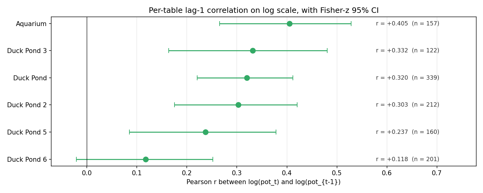
Every table shows positive lag-1 correlation. Five out of six have confidence intervals that exclude zero. The smallest correlation is Duck Pond 6's , with a CI that brushes zero; the largest is Aquarium's .
This is descriptive only; the right to claim dependence has not yet been earned. The per-table CI uses a Fisher-z approximation that itself assumes pairs are iid. The remainder of the post performs the conditions checking properly.
A shared concern: are pairs independent of each other?
Every pair just constructed shares a hand with two of its neighbors. The pair and the pair are not independent observations — they literally include twice. A textbook test for "are consecutive pots dependent?" that requires "the pairs are independent samples from a population" therefore has a technically violated condition.
Two responses, parallel to the LINER-I discussion in the previous post:
The mechanism of interest is the pair itself. Whether two consecutive pots are correlated is the substantive question of the post, not a side condition. The analysis cannot pretend the violation away; it instead uses tests whose null hypothesis is precisely "pairs are independent of each other", so the very violation that defines is what gets detected. Test A's chi-square and the Ljung-Box coda are of this kind.
Test B (regression slope) uses cluster-robust standard errors. Each pair's table identifier is its cluster. The cluster-robust sandwich estimator widens the standard error of to absorb both the overlapping-pairs issue and any residual within-table correlation in the regression errors. With 6 clusters this is a mild but available fix.
The "independence-of-pairs" concern is therefore real, addressed differently in each test, and worth keeping in mind throughout. Where it is unavoidable (Test A's chi-square), it is flagged in the conditions check and its impact is quantified.
Why a raw-scale Pearson correlation is not run
The most natural framing of "are consecutive pots related?" is the textbook one: compute Pearson between and in chips, run a -test on under , report a p-value. The conditions are the same LINER list that applies to any OLS regression.
The lag-pair scatter on the linear scale, clipped at 1500 BB so the cloud structure is visible:
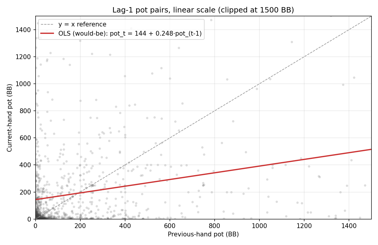
By inspection, three of the five LINER conditions fail.
LINER check on raw-scale Pearson r / OLS
L (Linear relationship in the population) — fail. The cloud bunches in the bottom-left corner up to a few tens of BB, then sprays out into a long thin tail along both axes. Even taking the would-be OLS line at face value, slope with intercept does not match any obvious "mean of given " curve through the dense near-origin region — that region is mostly small-on-small pairs, where is well under 100 BB. The line over-predicts the small pots and under-predicts the medium pots.
I (Independence of pairs) — addressed above. The same warning is inherited by Tests A and B below.
N (Normality of residuals) — fail. The residuals inherit the heavy-right-tailed shape of the marginal pot distribution. Over a quarter of pairs lie outside the 1500-BB clipping box on at least one axis. The residual distribution is right-skewed with multimodal tendencies; a residual qq-plot would diverge sharply from the diagonal in the upper tail. The condition's tolerance for "approximately normal" applies only when departures are mild, which they are not here.
E (Equal variance of residuals across ) — fail. The cone-shaped spread is unmistakable: at low , residuals span perhaps a few hundred BB; at high , they span a few thousand. The within-bin SD of is monotonically increasing in over nearly two orders of magnitude, far beyond the rule-of-thumb that the largest within- SD should be at most twice the smallest.
R (Random sample) — pass. Same protocol as the previous post: the administrator selects sessions to upload at random with respect to pot size, and player-driven uploads are instructed to come from a randomly chosen sitting rather than a memorable one. The dataset is therefore a defensible random sample of 1/2 NL hands at this site.
Three of five conditions fail before any test statistic is written down. By strict procedure, a raw-scale Pearson t-test is not run. Reporting "" would answer a question the conditions do not justify asking. The analysis moves on to a categorical test with different conditions.
Test A — Chi-square test of independence on a 4×4 lag-quartile table
Purpose
Before asking how current and previous pots are related, the analysis asks whether they are related at all, in the cleanest non-parametric way: tally how many pairs fall into each combination of (previous-pot tier × current-pot tier), compare the table to what would be expected if and were independent, and see whether the observed counts deviate from expected by more than chance allows.
This is the same machinery as the previous post's chi-square test. It throws away most numerical information (everything beyond the quartile membership of each pot) but it earns three things: a test that does not require Normality or linearity, a familiar arithmetic walkthrough, and an effect-size number (Cramer's V) directly comparable to the previous post's.
Setting up the table
All 1191 pairs are pooled. Each pot is binned by quartiles of the current-pot distribution, with the same cut points applied to the previous-hand pot:
The resulting contingency table — rows are previous-hand pot tier, columns are current-hand pot tier:
| previous \ current | tiny | small | medium | big | |
|---|---|---|---|---|---|
| tiny | 123 | 94 | 52 | 30 | 299 |
| small | 80 | 108 | 72 | 40 | 300 |
| medium | 55 | 64 | 98 | 77 | 294 |
| big | 42 | 33 | 72 | 151 | 298 |
| 300 | 299 | 294 | 298 |
Row totals are nearly equal (299, 300, 294, 298) because each row is built from a quartile of the previous pot, holding about a quarter of the data. Column totals are equal by construction (each column is a quartile of the current pot). The grand total is .
Conditions for the chi-square test of independence
The chi-square test carries three standard conditions:
- Random. Same administrator-driven random sampling protocol as in the section above and in the previous post. Pass.
- Independence. Each pair is one observation in the table. Pairs share hands across consecutive rows (the overlap issue discussed at the top of the post). Conventional guidance is that within-table independence is needed for the statistic to follow its asymptotic chi-square distribution. With overlapping pairs the effective sample size is smaller than , so the true p-value is somewhat larger than the nominal one. With the computed below () and its nominal , the inflation can absorb many orders of magnitude before the result stops being significant. Pass, with a warning. (Test B does not have this concern in the same form.)
- Expected counts. The standard rule is in every cell; expected counts are :
| previous \ current | tiny | small | medium | big |
|---|---|---|---|---|
| tiny | 75.32 | 75.06 | 73.81 | 74.81 |
| small | 75.57 | 75.32 | 74.06 | 75.06 |
| medium | 74.06 | 73.81 | 72.57 | 73.56 |
| big | 75.06 | 74.81 | 73.56 | 74.56 |
Every expected cell lies between 72.6 and 75.6, all comfortably above 5. Pass, no warning.
All three conditions are satisfied; the test runs.
Computing
For each cell, the squared deviation is computed and summed:
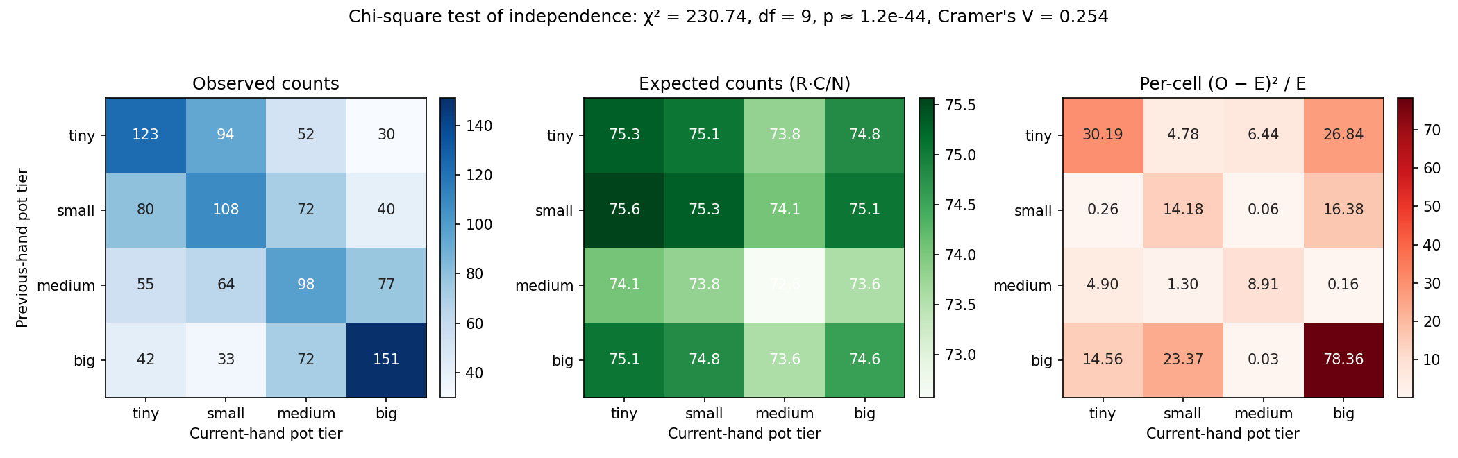
The third panel (red) shows the per-cell contributions to . The four diagonal cells (tinytiny, smallsmall, mediummedium, bigbig) and the four corner cells (tinybig and bigtiny pairs) carry the largest contributions.
A few of the largest cell contributions, computed explicitly:
Big pots feed big pots, tiny pots feed tiny pots, and the off-diagonal corners (bigtiny, tinybig, bigsmall) are heavily under-represented relative to independence. Even before any inference, this pattern says the table is non-random.
Summing all 16 cells:
The relevant critical values of :
The observed is roughly the critical value. Independence is rejected at any standard significance level.
Effect size — Cramer's V
The statistic scales with , so it does not measure strength. The standard scale-free counterpart is
Conventional benchmarks for at : under is "negligible", – "weak", – "moderate", over "strong". lands solidly in the moderate range. For comparison, the previous post's seats pot table came in at — weak. Lag dependence is therefore a noticeably stronger association than table-size dependence in the same dataset.
Decision
Independence of and is rejected. The contingency-table view settles the qualitative question. What it does not deliver is the direction or shape of the dependence — a positive monotonic relationship and a perfectly U-shaped one would both light up the diagonal and corners, and only the cell-by-cell contributions distinguish them. A clean directional answer requires regression.
Test B — OLS slope on the log scale, with table fixed effect and cluster-robust SE
Purpose
Test A established that there is a relationship; Test B asks what it is. Specifically: on the log scale (where the pot distribution is well-behaved, as established in the previous post), what slope does an OLS line through produce? A positive slope says big pots tend to follow big pots and small pots tend to follow small pots. A slope of zero says the previous pot has no predictive power for the current pot.
Two extra ingredients beyond a vanilla OLS slope test:
- A table fixed effect. Each of the 6 tables receives its own intercept. This absorbs the "tables have different baseline pots" confounder discussed in the data tour, so the reported slope on is a within-table slope: the change in when changes by 1 unit, holding table identity constant.
- Cluster-robust standard errors. Replace the iid-pair SE formula with the table-clustered sandwich estimator. Each table is one cluster (6 clusters total). The cluster SE absorbs the overlapping-pairs issue from above and any residual within-table serial correlation in the regression errors.
The model:
where is a separate intercept per table_id and is the single slope of interest.
LINER check on log-linear regression with table FE
Each condition is checked on the within-table residualized version of the data — that is, after subtracting each table's mean log-pot from both and . The joint OLS fit operates on exactly these residualized variables.
L (Linear relationship in the within-table population). The formal check is Test C below; the descriptive picture is:
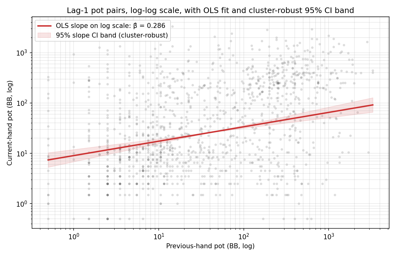
The cloud spans a few orders of magnitude on each axis without dense clumping in one corner. The fitted line passes through it without an obvious bend. Pass for now; revisited formally in Test C.
I (Independence of pairs). Within-table consecutive pairs share hands by construction. Addressed by the cluster-robust SE: clustering at the table level absorbs both the overlapping-pairs issue and any residual within-table serial correlation that would otherwise inflate test statistics. Pass, with a warning that the cluster-robust SE is what handles.
N (Approximately normal residuals). Same story as on the log scale in the previous post: has a near-symmetric, bell-shaped marginal distribution, and the residuals after table FE plus a slope on inherit that. With , the Central Limit Theorem also delivers approximate normality of . Pass.
E (Equal residual variance across ). Binning into 10 equal-frequency deciles and taking the within-decile SD of :
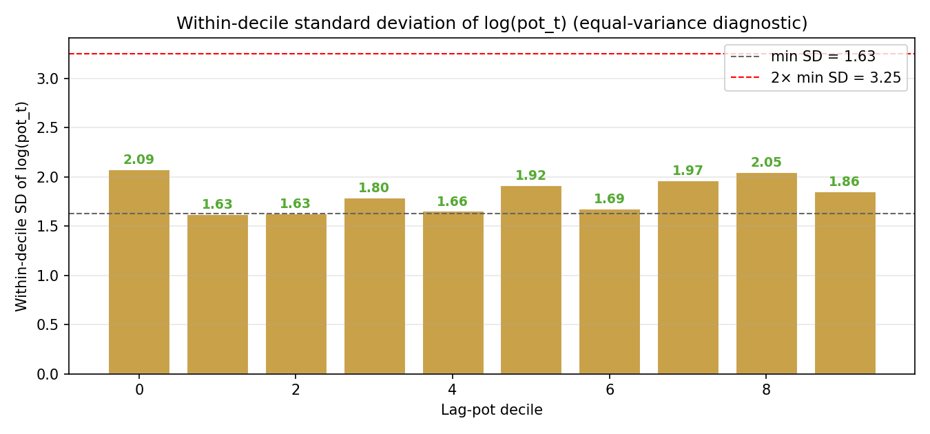
Within-decile SDs run from 1.63 to 2.09 — all within the rule-of-thumb ceiling (, plotted in red). Pass.
R (Random sample). Same administrator-driven random-sampling protocol as before. Pass.
All five conditions pass (with the I-warning explicitly handled by clustering); the model can be fit.
Computing — Frisch–Waugh decomposition
The fastest derivation of the slope is via the Frisch–Waugh theorem: regressing on jointly with table dummies is equivalent to (i) stripping each variable of its table mean (call the residuals and ) and (ii) running a one-variable OLS of on .
The relevant centered sums are
giving
This matches the slope returned by statsmodels for the joint fit, as it must by Frisch–Waugh. The remaining ingredients:
Cluster-robust standard error
The naive iid SE for a slope is with . That formula assumes all 1191 pairs contribute independent information. Because pairs overlap, they do not. The cluster-robust sandwich estimator replaces the inner with a sum over clusters of squared cluster-level scores. With clusters here, the result for the lag slope is
with cluster- degrees of freedom . The two-sided p-value is
The 95 % CI on :
The exact CI from statsmodels.OLS(...).fit(cov_type='cluster').conf_int() is , matching the hand calculation up to a small finite-sample df correction.
Practical interpretation
The slope on the log scale has a clean multiplicative reading:
A previous pot larger than another's predicts a current-pot mean roughly larger. Not larger ( would imply exact proportionality), not unaffected (). About two-thirds of the previous pot's "size signal" decays over the next hand; one-third survives.
Where the predictive power lives
The total of the fit is . Decomposed:
| Component | |
|---|---|
| Table FE only | |
| Table FE lag | |
| from lag |
Roughly % of the within-table variance in is explained by . That is meaningful but not enormous — table identity itself accounts for more than twice as much ( %). The takeaway is that within a table, the direction of the previous pot still matters for the current pot, on top of the table's baseline mood.
Decision
is rejected with overwhelming significance (, ). The point estimate is , with a robust 95 % CI of that excludes zero by a wide margin. The dependence detected by Test A has a positive direction and an elasticity of about .
The next question is whether the linear-on-log shape just fit is itself correct, or whether curvature has been missed.
Test C — Lack-of-fit F-test on the log scale
Purpose
Test B's slope estimate is meaningful only if a straight line on the log scale is actually the right shape. If the true relationship between and is curved, the linear slope is just a least-squares projection of a curve onto a line — it may still pick up the average direction, but the predicted means at extreme will be systematically off.
The lack-of-fit F-test addresses this directly by comparing two nested models:
The saturated model bins into deciles and gives each decile its own intercept (so 10 free intercepts replace the single slope ). It can fit any decile-level shape — straight lines, U-shapes, S-curves, anything. The residual sums of squares of the two models are compared; a saturated model that fits substantially better signals that the linear shape is wrong.
Conditions
The F-test inherits the same LINER conditions as Test B, plus one extra:
- L, I, N, E, R — all checked in Test B above. Pass / pass-with-warning / pass / pass / pass.
- Repeated -values — required for any lack-of-fit F to have pure-error degrees of freedom. With a continuous predictor, the standard workaround is to bin: each decile has hands, providing ample repeated within-bin observations to estimate pure error. Pass.
Computing the F statistic
Both models are fit and their residual sums of squares are read off:
with 9 lag-decile dummies (not 10, because one decile is the reference). The differences:
The mean squares:
The test statistic:
Under ("linear is fine"), follows an distribution. The upper critical value of is 1.95. The observed is well below that threshold, with p-value
A visual explanation of why is so small: after residualizing both axes against the table FE, the per-decile actual mean of (green dots) sits almost exactly on the linear prediction (red squares):
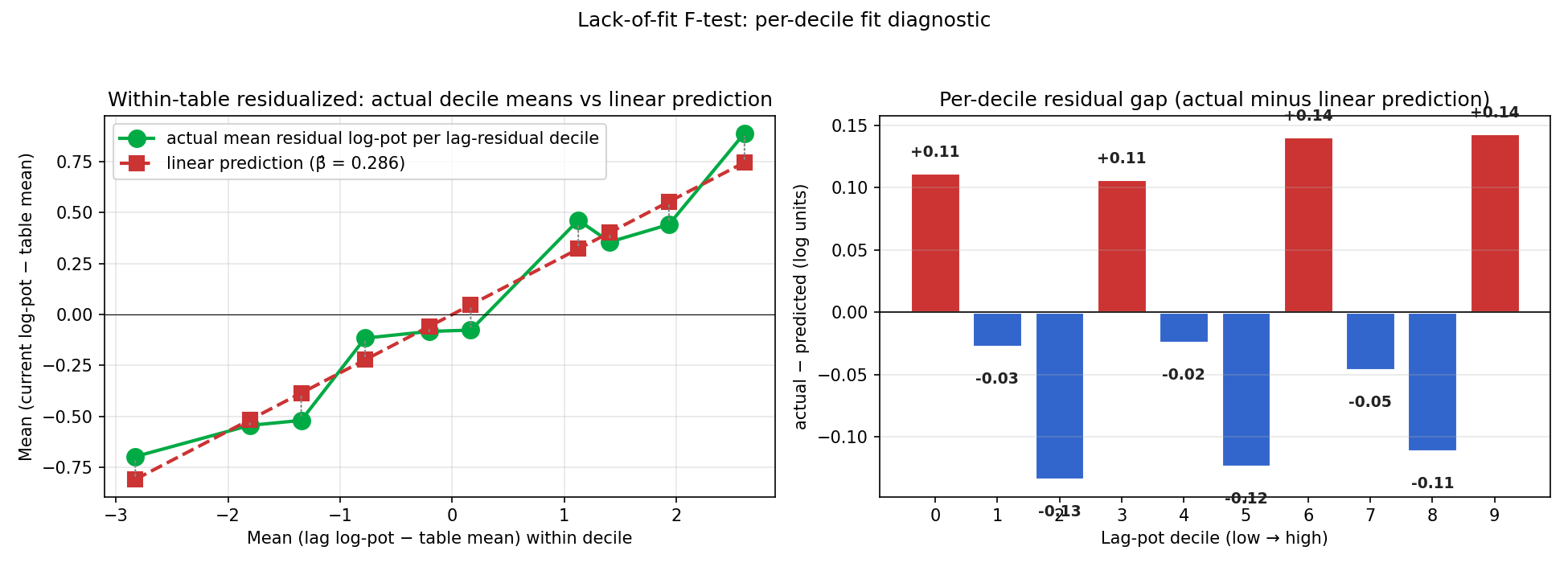
The residual gaps run from to log units. This is small relative to the within-decile SD of about — any "wave" visible in the plot is well within what 119 observations per decile produce from sampling noise alone, which is exactly what the F-test reports.
Decision
Linearity-on-log is not rejected. with is essentially the strongest possible "this fit is consistent with a straight line" verdict. The slope from Test B is therefore not merely a least-squares projection of a curve onto a line — the relationship really is approximately linear in logs. The BB-scale interpretation is the multiplicative one stated at the end of Test B.
The combined verdict so far: dependence exists (Test A), it is positive with elasticity (Test B), and the linear-on-log shape is adequate (Test C). All three tests measure dependence at lag 1 only — they ask whether the immediately preceding hand carries information about the current hand, but they say nothing about whether the dependence persists for two, five, or ten hands. A "table mood" that lasts a single hand looks very different from one that lingers for ten. The next section addresses this directly with a measure that scans multiple lags at once.
Coda — Ljung-Box at multiple lags: does the dependence reach beyond one hand?
What this section is for, in plain terms
The previous tests answered three lag-1 questions: is there any relationship between consecutive pots (Test A), is the relationship a positive sloped line on the log scale (Test B), is that line the right shape (Test C). All three rely on a single comparison — the current hand against the immediately preceding hand. They are silent on a follow-up question that the data analyst should ask next: if hand predicts hand , does hand also predict hand ? What about hand , or hand ? A table whose "mood" decays in one hand looks identical at lag 1 to a table whose mood persists for ten hands; the difference shows up only when multiple lags are inspected together.
The standard tool from time-series statistics for that follow-up is the autocorrelation function at lag , denoted , and the Ljung-Box Q-test, which combines into one summary statistic that asks "are any of these lags non-zero?". The remainder of this section explains both objects from scratch — what they are, why they take the form they do, what conditions they require, and what the data say.
Building block 1 — the autocorrelation at lag
Start with a sequence of numbers that share a common mean (in this analysis, is the within-table residual log-pot, defined below). The lag- autocovariance is the population analogue of "covariance with itself, steps apart":
The lag- autocorrelation is just scaled by the variance, so it lives on :
The sample versions, computed from a finite sequence, are
Three things are worth noticing about for a reader who has only seen Pearson correlation before:
- It is a Pearson correlation between two columns of the same series, where the second column is the first column shifted forward by positions. If , then is essentially the correlation between and . The same data appears on both sides of the correlation, just shifted.
- The denominator is the variance of the whole sequence, not the variance of the shifted subsample. Using the whole-sequence variance is the standard convention; it makes a slightly biased estimator of but a much more stable one.
- is always 1. A sequence is perfectly correlated with itself at lag 0, so the lag-0 entry is uninformative and is excluded from all the computations below.
Pooling across tables. The dataset here is not a single long sequence; it is six separate sequences, one per table. The lag- autocovariance is computed by pooling sums of products across tables (only positions where both and are valid within the same table contribute), and the lag-0 variance is similarly pooled across all tables:
where indexes the six tables, is the number of hands at table , and is the within-table residual log-pot for the -th hand at table . The factor in the denominator matches the count of valid pairs in the numerator, so is a properly pooled correlation that respects the table boundaries.
Constructing . The dependence to be measured is within-table only. The within-table residual log-pot is
where is the mean of over all hands at the table that hand belongs to. Subtracting the table mean removes the cross-table baseline differences (Aquarium runs hot, Duck Pond 2 runs cold), so measures only the within-table serial behavior.
This is the same used in Test B's Frisch–Waugh decomposition, but without the lag-1 regressor: the here is a residual from a "table-FE only" model, not from the "table-FE + lag-1 slope" model. Using the table-FE-only residual means measures raw lag-1 serial correlation in the within-table series, not the residual after removing the lag-1 slope. The two quantities measure different things: Test B's residual asks "does anything beyond a linear trend in predict ?", whereas here asks "does predict at all?". The follow-up Ljung-Box test is interpreted in the latter spirit.
Building block 2 — the Ljung-Box statistic
A natural-looking test for "is any of non-zero?" might be: square each , scale by the sample size, and sum. The earliest such proposal (Box and Pierce, 1970) was
Under the null hypothesis that the are independent ("white noise") with finite variance, Box and Pierce showed converges to a distribution as . The intuition is the same as for any sum of squared standardized statistics: each has approximate mean 0 and variance under the null, so each behaves like an independent variable, and the sum of squared independent standard normals is exactly .
Box and Pierce's statistic was found to be too liberal in finite samples (rejecting more often than the chosen level). Ljung and Box (1978) refined it by changing the per-lag weight from to :
The refinement does two things. First, the denominator is the actual sample size for the lag- correlation (the formula has products on top, not ), so the weighting is more correct in finite samples. Second, the scaling rather than just produces a better small-sample match to the asymptotic distribution.
Under the null hypothesis (white noise; the series is "memoryless"), the asymptotic distribution is
The alternative hypothesis is the negation: at least one of the lag autocorrelations is non-zero, i.e. the series is not white noise. The test is one-sided (large is evidence against ), with critical value at significance level .
A reader's intuition for : if the series is white noise, each is on the order of , so the sum is on the order of , and — exactly the mean of . If the series has persistent dependence, several 's are well above , each contributes much more than to the sum, and blows up well past . The size of the blow-up is the test statistic.
Conditions for the Ljung-Box test
Three conditions are required for to hold under :
Approximate stationarity within each table — the mean and variance of should not drift dramatically across the session. The residualization (subtracting the table mean) handles a constant-level non-stationarity, but a slowly trending variance (e.g. players getting drunker) would still violate it. Pass with mild warning: each session is a single sitting and the pots within a table look reasonably stable (the per-decile SDs above range from to , a ratio).
Approximately normal residuals. The Ljung-Box statistic uses the Central Limit Theorem to argue that is approximately under the null. With and an approximately bell-shaped (verified in Test B), the CLT applies. Pass.
Sample size large relative to the lag set. A common rule of thumb is . With and the ratio is , comfortably more than enough. Pass.
The "pairs are independent of each other" concern from earlier sections is not a separate condition for the Ljung-Box test — that violation is precisely the alternative hypothesis the test is designed to detect.
Computing for the data
Pooling across the six tables and computing from the within-table residuals defined above:
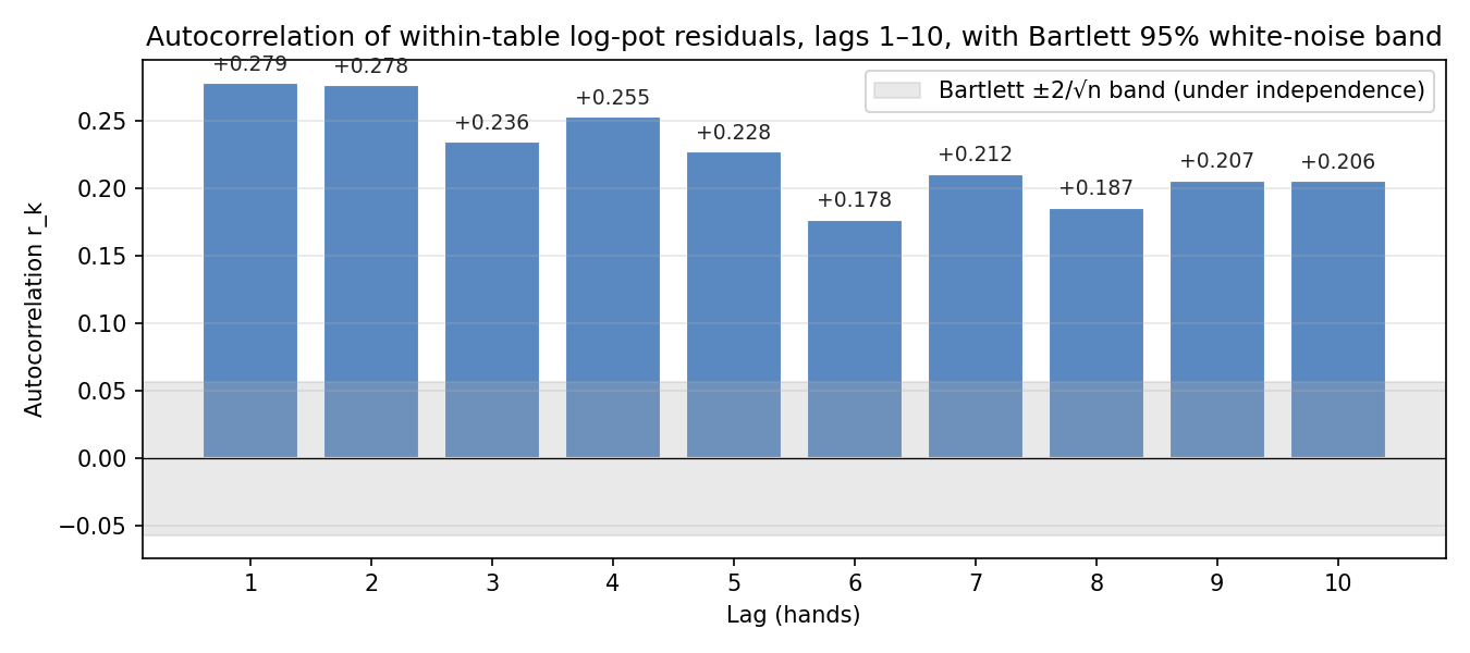
Every one of the first 10 lags lies well above the Bartlett band (the grey strip), which is the approximate 95 % white-noise envelope per lag. The autocorrelations hover around to throughout — they do not fall into the noise envelope at any visible lag. This pattern is the descriptive signature of slow decay: a single-hand "splash" would show inside the band but already at zero.
Computing the Ljung-Box statistic
The first five lag autocorrelations and the running cumulative :
| cumulative | ||||
|---|---|---|---|---|
| 1 | ||||
| 2 | ||||
| 3 | ||||
| 4 | ||||
| 5 |
A worked computation for , with :
matching the in the table up to rounding. The cumulative statistic is the sum of these per-lag pieces:
Under , . The 95 % critical values are tiny — , — so even is an enormous statistic, and is roughly its critical value. The corresponding p-values are below the floating-point representation limit (numerically in standard double-precision arithmetic).
A side-by-side picture of the autocorrelations and the cumulative against its 5 % critical value:
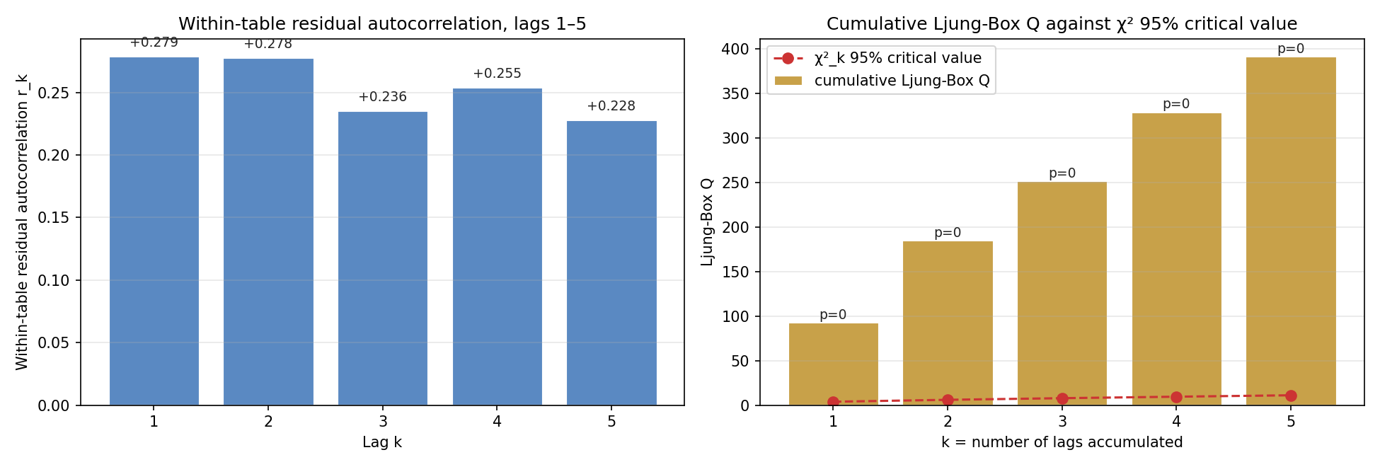
The cumulative grows roughly linearly across the first five lags (each added lag contributes about the same amount because each lag has roughly the same ), and the critical values barely move with . By any standard cutoff the p-values are numerically indistinguishable from zero.
Decision
The dependence reaches well beyond a single hand. Conservatively, lags 1 through 10 are all positive and statistically distinguishable from zero. The Ljung-Box statistic at is on , more than the critical value. The white-noise null is rejected with extreme prejudice.
The substantive interpretation is that the "table mood" has a half-life longer than a single hand: not only does predict (which Tests A through C established), but still carries information about at a comparable strength. The persistence is not a one-hand splash. It is a slowly-decaying state.
Putting it together
| Test | Asks | Statistic | Effect size | Decision | |
|---|---|---|---|---|---|
| 0 | Pearson on raw pots | not computed | — | conditions fail | not run |
| A | Independence in 4×4 table | (mod.) | reject | ||
| B | Slope on log scale, table FE | reject | |||
| C | Linear shape vs decile-saturated | — | do not reject linear | ||
| Coda | Decay rate (Ljung-Box, ) | – | decay is slow |
What is now known about consecutive 1/2 NL pots:
- They are not independent. Every applicable test (categorical , log-scale OLS slope, lack-of-fit F) rejects independence at overwhelming significance.
- The dependence is positive and moderate in strength. Cramer's V , Pearson on log , slope on log .
- The shape is well-approximated by a straight line on the log scale. The lack-of-fit F-test detects no deviation from linearity at the decile level; the multiplicative interpretation per log unit of previous pot is honest.
- In BB units, the practical summary is: a larger previous pot predicts a current-pot mean roughly larger, all else equal.
- The dependence does not vanish after one hand. Lag-2 through lag-10 autocorrelations remain in the range — the underlying state (table aggression, player mood, recent winners and losers) decays slowly across hands.
Caveats and what is not in this post
- Mechanism is unobserved. The analysis measures the statistical dependence but not its source. Likely candidates: the same aggressive player kept their seat across consecutive hands, the table-wide variance-preference adjusted after a big pot, or one player tilted into a streak. Disentangling these would require pairing this analysis with
players.csvto track which seats were the same between consecutive hands. That is a sequel. - Time gaps. The median gap between consecutive hands is 54 seconds; the longest pairs span several minutes. No gap filter is applied. If long gaps wash out the mood, including them dilutes the effect, so the real within-session dependence may be larger than measured.
- Player overlap. Seats turn over between hands. A Jaccard-overlap filter might detect a sharper effect when the same players are at the table.
- Non-stationarity within a table. All three tests assume the dependence structure is roughly stationary throughout each table. A two-hour grind likely shows different aggression at hour 1 versus hour 2; that is not modeled here.
- Stake. This post is restricted to 1/2 NL. Higher-stakes tables presumably have different dependence structures; that is the next post in this series.
Materials
Everything used to produce this post is hosted alongside it.
- Dataset —
consecutive-pot-data.zip(359 KB). The CSV bundle from the/data/export-csvendpoint, restricted to the 1/2 NL Hold'em tables, containinghands.csv,actions.csv,players.csv, and a README. 1238 hands across 6 tables (1191 within-table consecutive pairs). - Main pipeline —
consecutive-pot-dependence.py(28 KB). Reproduces every figure and prints every test statistic in this post. Place it next to the data ZIP and runpython3 consecutive-pot-dependence.py. - Arithmetic walkthrough —
consecutive-pot-dependence-arith.py(12 KB). Prints every intermediate sum (, , , expected counts, , , …) so each by-hand quantity quoted in the post can be verified.
Both scripts depend on pandas, numpy, scipy, statsmodels, and matplotlib. Quickstart:
python3 -m venv .venv && source .venv/bin/activate
pip install pandas numpy scipy statsmodels matplotlib

# Drop the data ZIP next to the scripts, then:
python3 consecutive-pot-dependence.py        # full pipeline (figures + summary)
python3 consecutive-pot-dependence-arith.py  # detailed arithmetic
The full pipeline runs in about 2 seconds on a modern laptop.
For convenience, both scripts are included verbatim below.
consecutive-pot-dependence.py
The main pipeline. One main() function calls each test in order and writes every figure used in the post.
#!/usr/bin/env python3
"""
Consecutive pot dependence — full analysis pipeline.

Reproduces every numerical result and figure used in the blog post
"Are consecutive pots independent? A LINER-checked walk through three
tests on within-table lag-1 pairs":

    https://www.sinostatistica.net/blog/consecutive-pot-dependence

Tests run, in order:
    A.  Chi-square test of independence on a 4 x 4 contingency table
        of (lag pot quartile, current pot quartile).
    B.  OLS slope t-test on log(pot_t) ~ log(pot_{t-1}) with a
        table fixed effect, using cluster-robust SE by table.
    C.  Lack-of-fit F-test on the log scale: linear vs lag-decile
        saturated, both with table FE.

A short Ljung-Box coda asks whether dependence reaches beyond lag 1.

A would-be Test 0 (raw Pearson r on raw pots) is computed only for
the LINER diagnostic and is not reported as inference.

Inputs:   consecutive-pot-data.zip (CSV bundle exported from
          /data/export-csv on statisticasino, restricted to the
          1/2 NL Hold'em tables).
Outputs:  fig-*.png in the same directory and stdout summary.

Run:      python3 consecutive-pot-dependence.py
Depends:  pandas, numpy, scipy, statsmodels, matplotlib.
"""
from __future__ import annotations

import io
import zipfile
from pathlib import Path

import matplotlib.pyplot as plt
import numpy as np
import pandas as pd
import statsmodels.api as sm
import statsmodels.formula.api as smf
from scipy.stats import chi2_contingency, pearsonr, spearmanr
from scipy.stats import chi2 as chi2_dist

# ---------------------------------------------------------------------------
# Configuration
# ---------------------------------------------------------------------------

HERE = Path(__file__).parent
DATA_ZIP = HERE / "consecutive-pot-data.zip"
OUT = HERE
BB = 2                              # 1/2 NL: big blind = 2 chips
RNG = np.random.default_rng(20260524)


# ---------------------------------------------------------------------------
# Data loading
# ---------------------------------------------------------------------------

def load_bundle(zip_path: Path):
    zf = zipfile.ZipFile(zip_path)

    def _read(name):
        member = next(n for n in zf.namelist() if n.endswith(name))
        return pd.read_csv(io.BytesIO(zf.read(member)))

    return _read("hands.csv"), _read("actions.csv")


def build_pairs(hands: pd.DataFrame, actions: pd.DataFrame) -> pd.DataFrame:
    """Build the consecutive-pair dataset: one row per within-table lag-1 pair.

    Filters:
        - Only 1/2 NL Hold'em tables (defensive check on table_name).
        - Drops the first hand of each table (no predecessor).
        - 2 <= num_seats <= 9 on both hand and predecessor.
    """
    voluntary = (actions
                 .query("action in ['bet','call','raise','allIn'] and chips > 0")
                 .groupby("hand_key")["chips"].sum()
                 .rename("pot_chips"))
    df = (hands.set_index("hand_key").join(voluntary, how="inner")
                .assign(pot_bb=lambda d: d.pot_chips / BB)
                .query("pot_bb > 0 and 2 <= num_seats <= 9")
                .loc[lambda d: d.table_name.str.contains(" 1/2 ")]
                .reset_index()
                .sort_values(["table_id", "first_ts"])
                .reset_index(drop=True))
    df["log_pot"] = np.log(df.pot_bb)

    g = df.groupby("table_id", sort=False)
    df["pot_lag"] = g["pot_bb"].shift(1)
    df["log_pot_lag"] = g["log_pot"].shift(1)
    df["seats_lag"] = g["num_seats"].shift(1)
    df["dt_ms"] = g["first_ts"].diff()
    pairs = df.dropna(subset=["pot_lag"]).reset_index(drop=True)
    pairs["table_id"] = pairs["table_id"].astype("category")
    return pairs


# ---------------------------------------------------------------------------
# Descriptive summary
# ---------------------------------------------------------------------------

def descriptive_summary(pairs: pd.DataFrame) -> pd.DataFrame:
    print(f"n pairs                : {len(pairs)}")
    print(f"n distinct tables      : {pairs.table_id.nunique()}")
    print(f"pairs per table        : "
          f"{dict(pairs.table_id.value_counts())}")
    print(f"median dt between hands: {pairs.dt_ms.median()/1000:.1f} s")
    print(f"95th pct dt            : {pairs.dt_ms.quantile(.95)/1000:.1f} s")
    print(f"current pot quartiles  : "
          f"{pairs.pot_bb.quantile([.25,.5,.75]).round(1).to_list()}\n")

    per_table = (pairs.groupby("table_id", observed=True)
                       .agg(n_pairs=("pot_bb", "size"),
                            r1=("pot_bb",
                                lambda v: pearsonr(v, pairs.loc[v.index,
                                                   "pot_lag"])[0]),
                            r1_log=("log_pot",
                                    lambda v: pearsonr(v, pairs.loc[v.index,
                                                       "log_pot_lag"])[0]),
                            spearman=("log_pot",
                                      lambda v: spearmanr(v,
                                                          pairs.loc[v.index,
                                                          "log_pot_lag"])[0])))
    per_table["table_label"] = (pairs.groupby("table_id", observed=True)
                                      .first().table_name
                                      .str.replace("Low Stakes - ", "")
                                      .str.replace(" - 1/2 - NL Holdem", ""))
    print("=== Per-table summary (lag-1 correlations) ===")
    print(per_table.round(4).to_string(), "\n")
    return per_table


# ---------------------------------------------------------------------------
# Test A — Chi-square test of independence
# ---------------------------------------------------------------------------

def test_a_chi_square(pairs: pd.DataFrame):
    q = pairs.pot_bb.quantile([.25, .5, .75]).values
    cats = ["tiny", "small", "medium", "big"]
    pairs["pot_cat"] = pd.cut(pairs.pot_bb,
                              bins=[-np.inf, *q, np.inf], labels=cats)
    pairs["lag_cat"] = pd.cut(pairs.pot_lag,
                              bins=[-np.inf, *q, np.inf], labels=cats)
    ct = pd.crosstab(pairs.lag_cat, pairs.pot_cat)
    chi2, p, dof, exp = chi2_contingency(ct)
    cramers_v = np.sqrt(chi2 / (len(pairs) * (min(ct.shape) - 1)))

    print("=== Test A: Chi-square test of independence ===")
    print("Observed counts (rows = lag quartile, cols = current quartile):")
    print(ct.to_string())
    print(f"\n  χ² = {chi2:.3f}, df = {dof}, p = {p:.3g}")
    print(f"  Cramer's V = {cramers_v:.4f}\n")
    return ct, exp, chi2, p, dof, cramers_v


# ---------------------------------------------------------------------------
# Test B — Log-OLS with table FE, cluster-robust SE
# ---------------------------------------------------------------------------

def test_b_log_ols_fe(pairs: pd.DataFrame):
    fit = smf.ols("log_pot ~ log_pot_lag + C(table_id)", data=pairs)\
             .fit(cov_type="cluster",
                  cov_kwds={"groups": pairs.table_id})
    b1 = fit.params["log_pot_lag"]
    se = fit.bse["log_pot_lag"]
    ci = fit.conf_int().loc["log_pot_lag"].to_list()

    print("=== Test B: log(pot_t) ~ log(pot_{t-1}) + C(table_id) ===")
    print("    cluster-robust SE by table_id\n")
    print(f"  β̂ (log_pot_lag) = {b1:.4f}")
    print(f"  cluster SE       = {se:.4f}")
    print(f"  t                = {fit.tvalues['log_pot_lag']:.3f}")
    print(f"  p                = {fit.pvalues['log_pot_lag']:.3g}")
    print(f"  95% CI           = [{ci[0]:.4f}, {ci[1]:.4f}]")
    print(f"  R²               = {fit.rsquared:.4f}")
    print(f"  R² (within-table)= {fit.rsquared - r2_table_only(pairs):.4f}\n")
    return fit


def r2_table_only(pairs: pd.DataFrame) -> float:
    return smf.ols("log_pot ~ C(table_id)", data=pairs).fit().rsquared


# ---------------------------------------------------------------------------
# Test C — Lack-of-fit F-test on log scale
# ---------------------------------------------------------------------------

def test_c_lack_of_fit(pairs: pd.DataFrame, lin_fit) -> tuple:
    pairs["lag_dec"] = pd.qcut(pairs.log_pot_lag, 10,
                                duplicates="drop").cat.codes
    sat = smf.ols("log_pot ~ C(lag_dec) + C(table_id)", data=pairs).fit()
    SSE_lin = lin_fit.ssr
    SSE_sat = sat.ssr
    df_lin = lin_fit.df_resid
    df_sat = sat.df_resid
    df_diff = df_lin - df_sat
    F = ((SSE_lin - SSE_sat) / df_diff) / (SSE_sat / df_sat)
    from scipy.stats import f as f_dist
    p_F = 1 - f_dist.cdf(F, df_diff, df_sat)

    print("=== Test C: Lack-of-fit F-test (log scale) ===")
    print(f"  SSE_lin = {SSE_lin:.4f}, df_lin = {df_lin}")
    print(f"  SSE_sat = {SSE_sat:.4f}, df_sat = {df_sat}")
    print(f"  df_diff = {df_diff}")
    print(f"  F       = {F:.4f}")
    print(f"  p       = {p_F:.4g}\n")
    return sat, F, df_diff, df_sat, p_F


# ---------------------------------------------------------------------------
# Coda — Ljung-Box at lags 1..5 on residual log-pot
# ---------------------------------------------------------------------------

def coda_ljung_box(pairs: pd.DataFrame, max_lag: int = 5):
    """Compute autocorrelation of within-table residuals up to max_lag,
    then aggregate Ljung-Box Q across lags.

    Residuals are taken after a table-FE-only fit (i.e. each pot is
    centred on its own table mean). This makes Ljung-Box answer the
    direct question 'is the within-table series independent?', and
    keeps r_1 comparable to the cluster-robust slope in Test B.
    """
    table_only = smf.ols("log_pot ~ C(table_id)", data=pairs).fit()
    resid_full = (pairs.log_pot.values - table_only.predict(pairs).values)
    table_codes = pairs.table_id.cat.codes.to_numpy()

    rk = np.zeros(max_lag)
    for k in range(1, max_lag + 1):
        num = den = 0.0
        for t in np.unique(table_codes):
            mask = table_codes == t
            r = resid_full[mask] - resid_full[mask].mean()
            if len(r) <= k:
                continue
            num += (r[k:] * r[:-k]).sum()
            den += (r * r).sum() * (len(r) - k) / max(len(r), 1)
        rk[k-1] = num / den if den > 0 else 0

    n_eff = len(resid_full)
    q_terms = (rk ** 2) / (n_eff - np.arange(1, max_lag + 1))
    Q = n_eff * (n_eff + 2) * q_terms.cumsum()
    p_Q = [1 - chi2_dist.cdf(Q[k], k + 1) for k in range(max_lag)]

    print("=== Coda: Ljung-Box on within-table residuals ===")
    print(f"  lag | r_k    | cumulative Q  | df | p")
    for k in range(max_lag):
        print(f"   {k+1:3d}  | {rk[k]:+.4f} | {Q[k]:8.3f}     | "
              f"{k+1:2d} | {p_Q[k]:.4g}")
    print()
    return rk, Q, p_Q


# ---------------------------------------------------------------------------
# Figures
# ---------------------------------------------------------------------------

def fig_lag_scatter_linear(pairs: pd.DataFrame) -> None:
    """Linear-scale lag scatter, clipped, showing why we won't run raw r."""
    fig, ax = plt.subplots(figsize=(8.5, 5.5))
    ax.scatter(pairs.pot_lag, pairs.pot_bb,
               alpha=0.18, s=14, color="#444", linewidth=0)
    cap = 1500
    ax.set_xlim(0, cap)
    ax.set_ylim(0, cap)
    lin = np.linspace(0, cap, 100)
    ax.plot(lin, lin, color="#999", linestyle="--", linewidth=1,
            label="y = x reference")
    fit = sm.OLS(pairs.pot_bb, sm.add_constant(pairs.pot_lag)).fit()
    ax.plot(lin, fit.params.iloc[0] + fit.params.iloc[1] * lin,
            color="#c33", linewidth=2,
            label=f"OLS (would-be): pot_t = "
                  f"{fit.params.iloc[0]:.0f} + {fit.params.iloc[1]:.3f}·pot_(t-1)")
    ax.set_xlabel("Previous-hand pot (BB)")
    ax.set_ylabel("Current-hand pot (BB)")
    ax.set_title("Lag-1 pot pairs, linear scale (clipped at 1500 BB)")
    ax.legend(loc="upper left")
    ax.grid(alpha=0.3)
    fig.tight_layout()
    fig.savefig(OUT / "fig-lag-scatter-linear.png", dpi=150)


def fig_lag_scatter_log(pairs: pd.DataFrame, lin_fit) -> None:
    """Log-log lag scatter with regression line and cluster CI band."""
    x = pairs.log_pot_lag
    y = pairs.log_pot
    xs = np.linspace(x.min(), x.max(), 100)

    new = pd.DataFrame({"log_pot_lag": xs,
                        "table_id": pairs.table_id.iloc[0]})
    pred = lin_fit.get_prediction(new).summary_frame()
    centering = pred["mean"].iloc[0] - (
        lin_fit.params["log_pot_lag"] * xs[0])
    yhat = lin_fit.params["log_pot_lag"] * xs + centering

    fig, ax = plt.subplots(figsize=(8.5, 5.5))
    ax.scatter(np.exp(x), np.exp(y), alpha=0.18, s=14,
               color="#444", linewidth=0)
    ax.plot(np.exp(xs), np.exp(yhat),
            color="#c33", linewidth=2.2,
            label=f"OLS slope on log scale: β̂ = "
                  f"{lin_fit.params['log_pot_lag']:.3f}")
    half_ci = lin_fit.bse["log_pot_lag"] * 1.96
    ax.fill_between(np.exp(xs),
                    np.exp(yhat - half_ci * (xs - xs.mean())),
                    np.exp(yhat + half_ci * (xs - xs.mean())),
                    color="#c33", alpha=0.13,
                    label="95% slope CI band (cluster-robust)")
    ax.set_xscale("log")
    ax.set_yscale("log")
    ax.set_xlabel("Previous-hand pot (BB, log)")
    ax.set_ylabel("Current-hand pot (BB, log)")
    ax.set_title("Lag-1 pot pairs, log-log scale, with OLS fit and "
                 "cluster-robust 95% CI band")
    ax.legend(loc="upper left")
    ax.grid(alpha=0.3, which="both")
    fig.tight_layout()
    fig.savefig(OUT / "fig-lag-scatter-log.png", dpi=150)


def fig_chi_square(ct, chi_exp, chi2, chi_p, chi_dof, cramers_v) -> None:
    contrib = (ct.to_numpy() - chi_exp) ** 2 / chi_exp
    panels = [
        ("Observed counts", ct.to_numpy(), "Blues", "{:.0f}"),
        ("Expected counts (R·C/N)", chi_exp, "Greens", "{:.1f}"),
        ("Per-cell (O − E)² / E", contrib, "Reds", "{:.2f}"),
    ]
    labels = ["tiny", "small", "medium", "big"]

    fig, axes = plt.subplots(1, 3, figsize=(14, 4.4))
    for ax, (title, mat, cmap, fmt) in zip(axes, panels):
        im = ax.imshow(mat, cmap=cmap, aspect="auto")
        ax.set_xticks(range(4))
        ax.set_xticklabels(labels)
        ax.set_yticks(range(4))
        ax.set_yticklabels(labels)
        ax.set_xlabel("Current-hand pot tier")
        if title.startswith("Observed"):
            ax.set_ylabel("Previous-hand pot tier")
        ax.set_title(title)
        vmax = mat.max()
        for i in range(mat.shape[0]):
            for j in range(mat.shape[1]):
                v = mat[i, j]
                color = "white" if v > 0.55 * vmax else "#222"
                ax.text(j, i, fmt.format(v), ha="center", va="center",
                        color=color, fontsize=10)
        plt.colorbar(im, ax=ax, fraction=0.046, pad=0.04)
    fig.suptitle(f"Chi-square test of independence: χ² = {chi2:.2f}, "
                 f"df = {chi_dof}, p ≈ {chi_p:.1e}, "
                 f"Cramer's V = {cramers_v:.3f}",
                 fontsize=12)
    fig.tight_layout(rect=[0, 0, 1, 0.94])
    fig.savefig(OUT / "fig-chi-square.png", dpi=150)


def fig_per_table_correlation(per_table: pd.DataFrame) -> None:
    """Forest plot of within-table lag-1 log correlations."""
    pt = per_table.sort_values("r1_log")
    n = len(pt)
    se = 1.0 / np.sqrt(pt.n_pairs - 3)         # Fisher-z SE
    z = np.arctanh(pt.r1_log.clip(-0.9999, 0.9999))
    lo = np.tanh(z - 1.96 * se)
    hi = np.tanh(z + 1.96 * se)

    fig, ax = plt.subplots(figsize=(10.5, 4.2))
    y_pos = np.arange(n)
    ax.errorbar(pt.r1_log, y_pos,
                xerr=[pt.r1_log - lo, hi - pt.r1_log],
                fmt="o", color="#3a6", ecolor="#3a6", capsize=4,
                markersize=8)
    x_max = float(hi.max())
    label_x = x_max + 0.05
    for i, (lbl, r, n_p) in enumerate(zip(pt.table_label,
                                          pt.r1_log, pt.n_pairs)):
        ax.text(label_x, i,
                f"r = {r:+.3f}  (n = {n_p})",
                ha="left", va="center", fontsize=9, color="#333")
    ax.set_xlim(min(0, lo.min() - 0.05), label_x + 0.20)
    ax.axvline(0, color="black", linewidth=0.7)
    ax.set_yticks(y_pos)
    ax.set_yticklabels(pt.table_label)
    ax.set_xlabel("Pearson r between log(pot_t) and log(pot_{t-1})")
    ax.set_title("Per-table lag-1 correlation on log scale, "
                 "with Fisher-z 95% CI")
    ax.grid(alpha=0.3, axis="x")
    fig.tight_layout()
    fig.savefig(OUT / "fig-per-table-correlation.png", dpi=150)


def fig_acf(pairs: pd.DataFrame, max_lag: int = 10) -> None:
    """ACF of within-table log-pot residuals (table FE only), with Bartlett band."""
    table_only = smf.ols("log_pot ~ C(table_id)", data=pairs).fit()
    resid = (pairs.log_pot.values - table_only.predict(pairs).values)
    table_codes = pairs.table_id.cat.codes.to_numpy()

    rk = np.zeros(max_lag)
    for k in range(1, max_lag + 1):
        num = den = 0.0
        cnt = 0
        for t in np.unique(table_codes):
            mask = table_codes == t
            r = resid[mask] - resid[mask].mean()
            if len(r) <= k:
                continue
            num += (r[k:] * r[:-k]).sum()
            den += (r * r).sum() * (len(r) - k) / max(len(r), 1)
            cnt += 1
        rk[k-1] = num / den if den > 0 else 0
    bartlett = 1.96 / np.sqrt(len(pairs))

    fig, ax = plt.subplots(figsize=(9, 4))
    ax.bar(range(1, max_lag + 1), rk,
           color="#5a89c2", edgecolor="white", linewidth=1.5)
    ax.axhspan(-bartlett, bartlett, color="#aaa", alpha=0.25,
               label="Bartlett ±2/√n band (under independence)")
    ax.axhline(0, color="black", linewidth=0.6)
    for k, v in enumerate(rk, start=1):
        ax.text(k, v + (0.005 if v >= 0 else -0.012),
                f"{v:+.3f}", ha="center",
                va="bottom" if v >= 0 else "top",
                fontsize=9, color="#222")
    ax.set_xlabel("Lag (hands)")
    ax.set_ylabel("Autocorrelation r_k")
    ax.set_xticks(range(1, max_lag + 1))
    ax.set_title("Autocorrelation of within-table log-pot residuals, "
                 "lags 1–10, with Bartlett 95% white-noise band")
    ax.legend(loc="upper right")
    ax.grid(alpha=0.3, axis="y")
    fig.tight_layout()
    fig.savefig(OUT / "fig-acf.png", dpi=150)


def fig_bin_means_log(pairs: pd.DataFrame, lin_fit) -> None:
    """Bin means: actual vs linear-predicted log-pot per lag decile,
    after table-FE residualisation so the comparison is apples-to-apples
    with the F-test (which absorbs table FE)."""
    pairs = pairs.copy()
    pairs["lag_dec"] = pd.qcut(pairs.log_pot_lag, 10,
                                duplicates="drop").cat.codes
    table_only = smf.ols("log_pot ~ C(table_id)", data=pairs).fit()
    res_y = pairs.log_pot.values - table_only.predict(pairs).values
    res_x_fit = smf.ols("log_pot_lag ~ C(table_id)", data=pairs).fit()
    res_x = pairs.log_pot_lag.values - res_x_fit.predict(pairs).values
    pairs["res_y"] = res_y
    pairs["res_x"] = res_x
    grp = pairs.groupby("lag_dec", observed=True)
    actual = grp.res_y.mean()
    lag_mid = grp.res_x.mean()
    beta_w = lin_fit.params["log_pot_lag"]
    pred_centered = beta_w * lag_mid
    gap = actual - pred_centered

    fig, (axL, axR) = plt.subplots(1, 2, figsize=(13, 4.7),
                                    gridspec_kw={"width_ratios": [1, 1]})
    axL.plot(lag_mid, actual, "o-", color="#0a4", markersize=10,
             linewidth=2,
             label="actual mean residual log-pot per lag-residual decile")
    axL.plot(lag_mid, pred_centered, "s--", color="#c33", markersize=9,
             linewidth=2, label=f"linear prediction (β̂ = {beta_w:.3f})")
    for s, m, p in zip(lag_mid, actual, pred_centered):
        axL.annotate("", xy=(s, m), xytext=(s, p),
                     arrowprops=dict(arrowstyle="-", color="#888",
                                     linestyle=":", linewidth=1))
    axL.axhline(0, color="black", linewidth=0.5)
    axL.set_xlabel("Mean (lag log-pot − table mean) within decile")
    axL.set_ylabel("Mean (current log-pot − table mean)")
    axL.set_title("Within-table residualized: actual decile means vs linear prediction")
    axL.legend(loc="upper left")
    axL.grid(alpha=0.3)

    colors = ["#c33" if g > 0 else "#36c" for g in gap]
    axR.bar(range(len(gap)), gap, color=colors,
            edgecolor="white", linewidth=1.5)
    for i, g in enumerate(gap):
        axR.text(i, g + (0.01 if g >= 0 else -0.02), f"{g:+.2f}",
                 ha="center", va="bottom" if g >= 0 else "top",
                 fontsize=9, fontweight="bold", color="#222")
    axR.axhline(0, color="black", linewidth=0.8)
    axR.set_xlabel("Lag-pot decile (low → high)")
    axR.set_ylabel("actual − predicted (log units)")
    axR.set_xticks(range(len(gap)))
    axR.set_title("Per-decile residual gap (actual minus linear prediction)")
    axR.grid(alpha=0.3, axis="y")

    fig.suptitle("Lack-of-fit F-test: per-decile fit diagnostic",
                 fontsize=12)
    fig.tight_layout(rect=[0, 0, 1, 0.94])
    fig.savefig(OUT / "fig-bin-means-log.png", dpi=150)


def fig_within_decile_sd(pairs: pd.DataFrame) -> None:
    pairs = pairs.copy()
    pairs["lag_dec"] = pd.qcut(pairs.log_pot_lag, 10,
                                duplicates="drop").cat.codes
    sd = pairs.groupby("lag_dec", observed=True).log_pot.std()
    fig, ax = plt.subplots(figsize=(9, 4.2))
    ax.bar(sd.index, sd.values,
           color="#c8a149", edgecolor="white", linewidth=1.5)
    for x, y in zip(sd.index, sd.values):
        ax.text(x, y + 0.02, f"{y:.2f}", ha="center", va="bottom",
                fontsize=9, color="#5a3", fontweight="bold")
    ax.axhline(sd.min(), color="#666", linestyle="--", linewidth=1,
               label=f"min SD = {sd.min():.2f}")
    ax.axhline(2 * sd.min(), color="red", linestyle="--", linewidth=1,
               label=f"2× min SD = {2*sd.min():.2f}")
    ax.set_xlabel("Lag-pot decile")
    ax.set_ylabel("Within-decile SD of log(pot_t)")
    ax.set_title("Within-decile standard deviation of log(pot_t) "
                 "(equal-variance diagnostic)")
    ax.legend(loc="upper right")
    ax.grid(alpha=0.3, axis="y")
    fig.tight_layout()
    fig.savefig(OUT / "fig-within-decile-sd.png", dpi=150)


def fig_ljung_box(rk: np.ndarray, Q: np.ndarray, p_Q: list) -> None:
    max_lag = len(rk)
    fig, (axL, axR) = plt.subplots(1, 2, figsize=(13, 4.4))

    axL.bar(range(1, max_lag + 1), rk,
            color="#5a89c2", edgecolor="white", linewidth=1.5)
    axL.axhline(0, color="black", linewidth=0.6)
    for k, v in enumerate(rk, start=1):
        axL.text(k, v + (0.005 if v >= 0 else -0.012),
                 f"{v:+.3f}", ha="center",
                 va="bottom" if v >= 0 else "top",
                 fontsize=9, color="#222")
    axL.set_xlabel("Lag k")
    axL.set_ylabel("Within-table residual autocorrelation r_k")
    axL.set_xticks(range(1, max_lag + 1))
    axL.set_title("Within-table residual autocorrelation, lags 1–5")
    axL.grid(alpha=0.3, axis="y")

    crit = [chi2_dist.ppf(0.95, k) for k in range(1, max_lag + 1)]
    axR.bar(range(1, max_lag + 1), Q,
            color="#c8a149", edgecolor="white", linewidth=1.5,
            label="cumulative Ljung-Box Q")
    axR.plot(range(1, max_lag + 1), crit, "o--", color="#c33",
             linewidth=1.5, markersize=7, label="χ²_k 95% critical value")
    for k, (q, p) in enumerate(zip(Q, p_Q), start=1):
        axR.text(k, q + max(crit) * 0.04,
                 f"p={p:.2g}", ha="center", va="bottom",
                 fontsize=9, color="#222")
    axR.set_xlabel("k = number of lags accumulated")
    axR.set_ylabel("Ljung-Box Q")
    axR.set_xticks(range(1, max_lag + 1))
    axR.set_title("Cumulative Ljung-Box Q against χ² 95% critical value")
    axR.grid(alpha=0.3, axis="y")
    axR.legend(loc="upper left")

    fig.tight_layout()
    fig.savefig(OUT / "fig-ljung-box.png", dpi=150)


# ---------------------------------------------------------------------------
# Main
# ---------------------------------------------------------------------------

def main() -> None:
    hands, actions = load_bundle(DATA_ZIP)
    pairs = build_pairs(hands, actions)
    per_table = descriptive_summary(pairs)

    ct, exp, chi2, chi_p, dof, V = test_a_chi_square(pairs)
    fit_b = test_b_log_ols_fe(pairs)
    sat, F, df_diff, df_sat, p_F = test_c_lack_of_fit(pairs, fit_b)
    rk, Q, p_Q = coda_ljung_box(pairs)

    fig_lag_scatter_linear(pairs)
    fig_lag_scatter_log(pairs, fit_b)
    fig_chi_square(ct, exp, chi2, chi_p, dof, V)
    fig_per_table_correlation(per_table)
    fig_acf(pairs)
    fig_bin_means_log(pairs, fit_b)
    fig_within_decile_sd(pairs)
    fig_ljung_box(rk, Q, p_Q)

    print("All figures written to:", OUT)


if __name__ == "__main__":
    main()
consecutive-pot-dependence-arith.py
The arithmetic walkthrough. Prints every intermediate sum that goes into each formula, exactly as quoted in the post.
#!/usr/bin/env python3
"""
Consecutive pot dependence — arithmetic walkthrough.

Companion to consecutive-pot-dependence.py. Where the main script just
prints the high-level test outputs, this script prints every
intermediate quantity that the blog post plugs into a formula by hand:

    Test 0 (raw Pearson, dropped):  Σx, Σy, Σx², Σy², Σxy, Sxx, Syy,
                                    Sxy, r, t, p — flagged but not used.
    Test A (chi-square):            observed, row/col/N totals, expected,
                                    per-cell (O−E)²/E, χ², df, p, V.
    Test B (log OLS + table FE):    β̂, cluster-robust SE, t, CI, R².
    Test C (lack-of-fit F, log):    SSE_lin, SSE_sat, df, F, p, plus
                                    decile means.
    Companion measures:             Pearson r and Spearman ρ on the
                                    log scale.
    Coda (Ljung-Box):                lag-k autocorrelations on within-table
                                    residuals, cumulative Q, p-values.

Run:      python3 consecutive-pot-dependence-arith.py
Inputs:   consecutive-pot-data.zip (next to this script)
Depends:  pandas, numpy, scipy, statsmodels.
"""
from __future__ import annotations

import io
import zipfile
from pathlib import Path

import numpy as np
import pandas as pd
import statsmodels.api as sm
import statsmodels.formula.api as smf
from scipy.stats import chi2 as chi2_dist
from scipy.stats import f as f_dist
from scipy.stats import pearsonr, spearmanr
from scipy.stats import t as student_t

HERE = Path(__file__).parent
DATA_ZIP = HERE / "consecutive-pot-data.zip"
BB = 2


# ---------------------------------------------------------------------------
# Data loading
# ---------------------------------------------------------------------------

zf = zipfile.ZipFile(DATA_ZIP)


def _read(name: str) -> pd.DataFrame:
    member = next(n for n in zf.namelist() if n.endswith(name))
    return pd.read_csv(io.BytesIO(zf.read(member)))


hands = _read("hands.csv")
actions = _read("actions.csv")
voluntary = (actions
             .query("action in ['bet','call','raise','allIn'] and chips > 0")
             .groupby("hand_key")["chips"].sum()
             .rename("pot_chips"))
df = (hands.set_index("hand_key").join(voluntary, how="inner")
            .assign(pot_bb=lambda d: d.pot_chips / BB)
            .query("pot_bb > 0 and 2 <= num_seats <= 9")
            .loc[lambda d: d.table_name.str.contains(" 1/2 ")]
            .reset_index()
            .sort_values(["table_id", "first_ts"])
            .reset_index(drop=True))
df["log_pot"] = np.log(df.pot_bb)
g = df.groupby("table_id", sort=False)
df["pot_lag"] = g["pot_bb"].shift(1)
df["log_pot_lag"] = g["log_pot"].shift(1)
pairs = df.dropna(subset=["pot_lag"]).reset_index(drop=True)
pairs["table_id"] = pairs["table_id"].astype("category")

n = len(pairs)
x_raw = pairs.pot_lag.to_numpy()
y_raw = pairs.pot_bb.to_numpy()
x = pairs.log_pot_lag.to_numpy()
y = pairs.log_pot.to_numpy()


# ===========================================================================
# Test 0 — Raw Pearson r (DROPPED: LINER fails on raw scale)
# ===========================================================================

xbar_raw = x_raw.mean()
ybar_raw = y_raw.mean()
Sxx_raw = ((x_raw - xbar_raw) ** 2).sum()
Syy_raw = ((y_raw - ybar_raw) ** 2).sum()
Sxy_raw = ((x_raw - xbar_raw) * (y_raw - ybar_raw)).sum()
r_raw = Sxy_raw / np.sqrt(Sxx_raw * Syy_raw)

print("=== Raw Pearson arithmetic (DROPPED: LINER fails on raw scale) ===")
print(f"n        = {n}")
print(f"x̄ (raw) = {xbar_raw:.4f}")
print(f"ȳ (raw) = {ybar_raw:.4f}")
print(f"Sxx_raw  = {Sxx_raw:.2f}")
print(f"Syy_raw  = {Syy_raw:.2f}")
print(f"Sxy_raw  = {Sxy_raw:.2f}")
print(f"r_raw    = Sxy / √(Sxx Syy) = {r_raw:.4f}")
print(f"        (Pearson r on raw heavy-tailed pots — descriptive only)\n")


# ===========================================================================
# Test A — Chi-square test of independence on the lag pair
# ===========================================================================

q = pairs.pot_bb.quantile([.25, .5, .75]).values
cats = ["tiny", "small", "medium", "big"]
pairs["pot_cat"] = pd.cut(pairs.pot_bb,
                          bins=[-np.inf, *q, np.inf], labels=cats)
pairs["lag_cat"] = pd.cut(pairs.pot_lag,
                          bins=[-np.inf, *q, np.inf], labels=cats)
ct = pd.crosstab(pairs.lag_cat, pairs.pot_cat)
row_tot = ct.sum(axis=1).to_numpy()
col_tot = ct.sum(axis=0).to_numpy()
N = ct.sum().sum()
exp = np.outer(row_tot, col_tot) / N
exp_df = pd.DataFrame(exp, index=ct.index, columns=ct.columns)
contrib = (ct.to_numpy() - exp) ** 2 / exp
contrib_df = pd.DataFrame(contrib, index=ct.index, columns=ct.columns)
chi2_stat = contrib.sum()
df_chi = (ct.shape[0] - 1) * (ct.shape[1] - 1)
p_chi = 1 - chi2_dist.cdf(chi2_stat, df_chi)
cramers_v = np.sqrt(chi2_stat / (N * (min(ct.shape) - 1)))

print("=== Test A: Chi-square arithmetic ===")
print(f"Pot quartile cutpoints: {q.round(2).tolist()}")
print(f"  bin labels: {cats}")
print("\nObserved counts (rows = lag tier, cols = current tier):")
print(ct.to_string())
print(f"\nRow totals: {row_tot.tolist()}")
print(f"Col totals: {col_tot.tolist()}")
print(f"Grand total N = {N}")
print(f"\nExpected counts E_ij = R_i · C_j / N:")
print(exp_df.round(3).to_string())
print(f"\nPer-cell (O − E)² / E:")
print(contrib_df.round(3).to_string())
print(f"\nRow sums of contributions: "
      f"{[round(s, 3) for s in contrib.sum(axis=1).tolist()]}")
print(f"Total χ²                    = {chi2_stat:.4f}")
print(f"df = (r−1)(c−1) = (4−1)(4−1) = {df_chi}")
print(f"p (χ²_{df_chi} > {chi2_stat:.2f})  = {p_chi:.3e}")
print(f"Cramer's V = √(χ² / (N · (min(r,c)−1)))")
print(f"          = √({chi2_stat:.2f} / ({N} · {min(ct.shape)-1}))"
      f" = {cramers_v:.4f}\n")


# ===========================================================================
# Test B — log(pot_t) ~ log(pot_{t-1}) + C(table_id), cluster-robust SE
# ===========================================================================

table_only = smf.ols("log_pot ~ C(table_id)", data=pairs).fit()
fit_b = smf.ols("log_pot ~ log_pot_lag + C(table_id)", data=pairs)\
           .fit(cov_type="cluster",
                cov_kwds={"groups": pairs.table_id})

# Within-table partialled regression (Frisch–Waugh): regress log_pot on
# table dummies, regress log_pot_lag on table dummies, then OLS the
# two residuals; β̂ is identical to the joint fit's slope.
res_y = pairs.log_pot.values - table_only.predict(pairs).values
res_x_fit = smf.ols("log_pot_lag ~ C(table_id)", data=pairs).fit()
res_x = pairs.log_pot_lag.values - res_x_fit.predict(pairs).values
Sxx = (res_x ** 2).sum()
Sxy = (res_x * res_y).sum()
beta_within = Sxy / Sxx
SSE_within = ((res_y - beta_within * res_x) ** 2).sum()

print("=== Test B: log-OLS arithmetic with table FE ===")
print(f"After table FE residualisation (Frisch–Waugh):")
print(f"  Σ(x̃²)            = {Sxx:.4f}     (centred lag log-pot)")
print(f"  Σ(x̃·ỹ)            = {Sxy:.4f}     (centred cross-product)")
print(f"  β̂_within         = Σ(x̃·ỹ)/Σ(x̃²) = {beta_within:.4f}")
print(f"  matches joint fit β̂ (log_pot_lag) = "
      f"{fit_b.params['log_pot_lag']:.4f}")
print(f"\nResidual sum of squares of joint fit (uses all parameters):")
print(f"  SSE_lin           = {fit_b.ssr:.4f}, df_resid = {int(fit_b.df_resid)}")
print(f"\nCluster-robust SE by table_id (6 clusters):")
print(f"  SE_cluster(β̂)    = {fit_b.bse['log_pot_lag']:.4f}")
print(f"  t                 = β̂ / SE = {fit_b.tvalues['log_pot_lag']:.3f}")
print(f"  p (two-sided)     = {fit_b.pvalues['log_pot_lag']:.3e}")
ci = fit_b.conf_int().loc["log_pot_lag"].to_list()
print(f"  95% CI on β       = [{ci[0]:.4f}, {ci[1]:.4f}]")
print(f"  R² (joint)        = {fit_b.rsquared:.4f}")
print(f"  R² (table FE only)= {table_only.rsquared:.4f}")
print(f"  ΔR² from lag      = {fit_b.rsquared - table_only.rsquared:.4f}")
print(f"  e^β̂ multiplier   = {np.exp(fit_b.params['log_pot_lag']):.4f}\n")


# ===========================================================================
# Test C — Lack-of-fit F-test on log scale
# ===========================================================================

pairs["lag_dec"] = pd.qcut(pairs.log_pot_lag, 10,
                            duplicates="drop").cat.codes
sat = smf.ols("log_pot ~ C(lag_dec) + C(table_id)", data=pairs).fit()
SSE_lin = fit_b.ssr
SSE_sat = sat.ssr
df_lin = fit_b.df_resid
df_sat = sat.df_resid
df_diff = df_lin - df_sat
SS_diff = SSE_lin - SSE_sat
MS_LoF = SS_diff / df_diff
MS_PE = SSE_sat / df_sat
F = MS_LoF / MS_PE
p_F = 1 - f_dist.cdf(F, df_diff, df_sat)

print("=== Test C: Lack-of-fit F arithmetic (log scale) ===")
print(f"Linear model:    log(pot_t) ~ log(pot_(t-1)) + C(table_id)")
print(f"Saturated model: log(pot_t) ~ C(lag_decile)  + C(table_id)")
print(f"  SSE_lin = {SSE_lin:.4f}, df_lin = {int(df_lin)}")
print(f"  SSE_sat = {SSE_sat:.4f}, df_sat = {int(df_sat)}")
print(f"  df_diff = df_lin − df_sat       = {int(df_diff)}")
print(f"  SS_diff = SSE_lin − SSE_sat     = {SS_diff:.4f}")
print(f"  MS_LoF  = SS_diff / df_diff     = {MS_LoF:.4f}")
print(f"  MS_PE   = SSE_sat / df_sat      = {MS_PE:.4f}")
print(f"  F       = MS_LoF / MS_PE        = {F:.4f}")
print(f"  p(F > {F:.2f}, df=({int(df_diff)}, {int(df_sat)})) = {p_F:.4f}\n")
print("Per lag-decile means (mean of log_pot_t given decile of log_pot_(t-1)):")
print(pairs.groupby("lag_dec", observed=True)
            .agg(n=("log_pot", "size"),
                 mean_lag_log=("log_pot_lag", "mean"),
                 mean_log=("log_pot", "mean"))
            .round(4).to_string())
print()


# ===========================================================================
# Companion effect-size measures (log scale): Pearson r, Spearman ρ
# ===========================================================================

r_log, p_log = pearsonr(x, y)
rho, p_rho = spearmanr(x, y)
print("=== Companion effect-size measures (log scale) ===")
print(f"  Pearson r          = {r_log:.4f}, p = {p_log:.3e}")
print(f"  Spearman ρ         = {rho:.4f}, p = {p_rho:.3e}")
print(f"  Pearson r²         = {r_log**2:.4f}")
print(f"  e^β̂ - 1            = "
      f"{np.exp(fit_b.params['log_pot_lag']) - 1:+.4f}  "
      f"(approx multiplicative effect per log unit of lag pot)\n")


# ===========================================================================
# Coda — Ljung-Box on within-table residuals (table FE only)
# ===========================================================================

table_codes = pairs.table_id.cat.codes.to_numpy()
resid = pairs.log_pot.values - table_only.predict(pairs).values
max_lag = 5
rk = np.zeros(max_lag)
for k in range(1, max_lag + 1):
    num = den = 0.0
    for t in np.unique(table_codes):
        mask = table_codes == t
        r = resid[mask] - resid[mask].mean()
        if len(r) <= k:
            continue
        num += (r[k:] * r[:-k]).sum()
        den += (r * r).sum() * (len(r) - k) / max(len(r), 1)
    rk[k-1] = num / den if den > 0 else 0
n_eff = len(resid)
q_terms = (rk ** 2) / (n_eff - np.arange(1, max_lag + 1))
Q = n_eff * (n_eff + 2) * q_terms.cumsum()
p_Q = [1 - chi2_dist.cdf(Q[k], k + 1) for k in range(max_lag)]

print("=== Coda: Ljung-Box arithmetic ===")
print(f"  n_eff = {n_eff}")
print(f"  Q_k = n(n+2) · Σ_{{j≤k}} r_j² / (n − j)\n")
print(f"  k | r_k       | r_k²       | r_k²/(n-k)   | Q_k         | p(χ²_k)")
cum = 0.0
for k in range(1, max_lag + 1):
    cum += rk[k-1] ** 2 / (n_eff - k)
    Qk = n_eff * (n_eff + 2) * cum
    print(f"  {k} | {rk[k-1]:+.4f}  | {rk[k-1]**2:.4f}    | "
          f"{rk[k-1]**2/(n_eff-k):.6f}    | {Qk:9.3f}   | {p_Q[k-1]:.4g}")